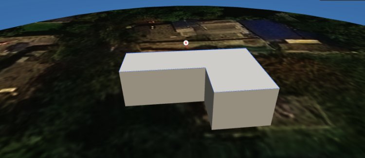
Metric Building-Layout Drawing for 3D Shadow Analysis in IST PVSolar Simulator V9.0.14

Abstract

Rooftop shading results are only as good as the building outline they are computed on. This article describes the metric layout-drawing method that IST PVSolar Simulator V9.0.14 uses to define the house footprint for its 3D shadow analysis, and validates it against closed-form geometry.

Walls are entered as length–bearing pairs in a local east–north frame with north fixed upward, using line, circular-arc and rectangle primitives together with snapping, trimming and constraint editing. A degree-two graph traversal closes the outline. The footprint is then transferred to the simulation as an exact-scale raster map and a floating-point roof polygon, and extruded to a 3D building. The building orientation is estimated by a length-weighted circular mean on quadrupled wall bearings, which sets the sun-facing façade and the module azimuth.

For an L-shaped reference house (20 m × 12 m with a 12 m × 6 m corner removed), the drawn and simulated footprint area was 168.00 m², matching the analytical value, with an interior-angle sum of 720° and a building angle of 0.0° from north. A 60′-6″ × 40′ house entered in feet transferred as 224.825 m² against an exact 224.825 m². A 10 m chord with 3 m sagitta produced a radius of 5.667 m (analytical 5.667 m), with a maximum chord-to-arc deviation of about 1.4 mm. Typed dimensions therefore introduce no measurable error into the simulation footprint; mouse-placed dimensions are bounded by the 0.5 m grid and 0.5° angular quantisation. The method removes the dependence on drone or satellite imagery for buildings whose dimensions are known from a site survey.

1. Introduction

The building footprint is the boundary condition for every rooftop shading calculation. It fixes the usable roof area, the position of parapets and rooftop obstructions, the distance to neighbouring objects, and the orientation of the module rows. An error in a wall length moves the roof edge; an error in the wall bearing rotates every array and changes its azimuth relative to the sun.

In image-based workflows the footprint is traced over a drone orthomosaic or satellite map. That approach inherits the image's limits: its ground sampling distance, its georeferencing and north alignment, roof overhangs that hide the true wall line, and tree canopy or shadow over the edges. Many rooftop projects also start before any image exists, with only a site survey of wall lengths and directions.

IST PVSolar Simulator V9.0.14 therefore offers a second route, Draw Building Plan, inside its 3D Shadow Analysis module. The engineer enters the house exactly as it is surveyed, wall by wall, as a length and a bearing from north. This article makes four contributions:

1. A formal description of the drawing model: coordinate frame, geometric primitives, snapping and constraint rules, and outline closure.
2. The transfer of the drawn footprint into the simulation: exact-scale rasterisation, the floating-point roof polygon, 3D extrusion and the derivation of building orientation and module azimuth.
3. A validation on reference houses with closed-form answers, in metres and in feet.
4. An error budget that separates typed dimensions, which are exact, from mouse-placed dimensions and arc discretisation, which are bounded.

2. System overview

The drawn house passes through four stages before any shading is computed: entry, closure, transfer and 3D modelling. At Apply, the transfer stage splits into three outputs that the shading engine consumes together.

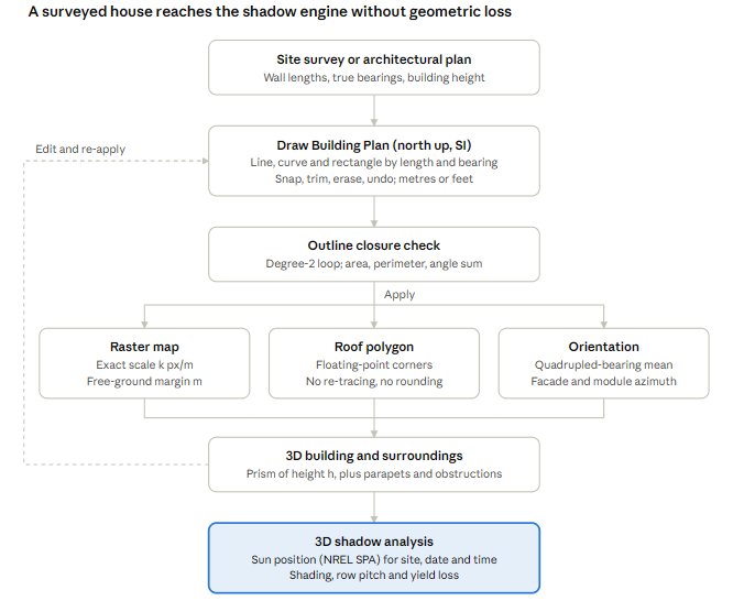
The roof polygon is passed as exact coordinates rather than re-traced from the raster map, which is why the transfer adds no geometric error (Section 5). The dashed path shows that a saved drawing can be reopened, edited and applied again at any time.

3. Methods

3.1 Coordinate frame and conventions

The house is drawn in a local, flat east–north frame: x points east, y points north, and all lengths are stored in metres. North is fixed to the top of the drawing and of every downstream map. A wall direction is a compass bearing β in degrees, measured clockwise from north (0° north, 90° east, 180° south, 270° west). A wall of length L starting at P₀ ends at

When a wall follows another with bearing βₖ₋₁, the corner angle shown live while drawing is

so a straight continuation reads 180° and a square corner 90°.

3.2 Geometric primitives

Line. The start point is clicked or snapped. The length L is then typed, and the bearing is either typed or taken from the cursor direction. The next wall starts at the end of the previous one, so a closed outline is a chain of length–bearing pairs, as in a traverse survey.

Circular arc. An arc is defined by its chord from P₀ to P₁ (entered like a line, length c and bearing) and a signed sagitta s, positive to the left of P₀→P₁. The bulge point is P_b = M + s·n, with M the chord midpoint and n the left unit normal. The arc is the circle through P₀, P_b and P₁, whose radius is

If the user types a radius R ≥ c/2 instead, the minor-arc sagitta is used, with its side taken from the cursor:

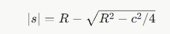
The sweep direction is the one that passes through P_b. The arc is stored as a polyline of n segments, with n = min(360, max(8, ⌈|Θ| r / 0.25 m⌉, ⌈|Θ| / 4°⌉)) for a sweep Θ, so every segment is at most 0.25 m long and spans at most 4°.

Rectangle. A first corner, a width and bearing for the first side, then a signed depth d along its left normal, give four line primitives.

3.3 Snapping and constraints

A cursor position is resolved in priority order: a wall end point within 11 screen pixels, then a wall midpoint, then the grid (default 0.5 m, or 1 ft in feet mode). Two points closer than ε = 0.02 m are treated as the same corner. Cursor bearings are quantised to 0.5° and are attracted within 1.5° to the four cardinal directions and to the previous wall's bearing plus multiples of 90°; holding Shift quantises to 15°. Typed lengths, bearings and radii bypass all quantisation and are used to full floating-point precision.

In the Select tool, editing a wall's length or bearing moves its end node, and every wall end that coincides with that node (within ε) moves with it, so connectivity is preserved. An arc whose end is moved is refitted with the same ratio of sagitta to chord.

3.4 Topology: trimming and outline closure

Trim. For a picked wall, all proper intersections with other walls are found from the parametric form of each segment pair, accepting parameters t, u ∈ [0, 1]. The intersections are expressed as distances along the wall, and the interval that contains the pick point is removed, leaving zero, one or two pieces.

Closure. Wall end points are merged into nodes within ε, giving a graph whose edges are the walls. Nodes of degree 1 are open ends and are flagged to the user. A closed outline is a connected component in which every node has degree 2; it is traversed to an ordered vertex list, and components enclosing less than 0.5 m² are discarded. When several closed outlines exist, the one with the largest enclosed area is taken as the building. Vertices that lie on a straight wall (zero cross product within tolerance) are removed before transfer.

3.5 Metric properties

The enclosed area A uses the shoelace (surveyor's) formula [3], whose sign also gives the vertex orientation, and the perimeter P is the sum of edge lengths:

The interior angle at vertex vᵢ is tᵢ = (β(vᵢ→vᵢ₊₁) − β(vᵢ→vᵢ₋₁)) mod 360°, replaced by 360° − tᵢ when A < 0. The interior angles of a valid simple outline sum to (n − 2)·180°, which serves as a consistency check.

3.6 Length units

All geometry is stored in SI. In feet mode, a typed length is parsed as decimal feet or as feet and inches, L = (F + I/12) × 0.3048 m, so 60'6" and 60.5 give the same 18.4404 m. Areas are converted with 1 ft² = 0.09290304 m². Lengths in feet are displayed rounded to the nearest half inch. This rounding is display-only, so switching units never alters the stored drawing.

3.7 Transfer to the simulation

On Apply, the outline's bounding box is enlarged by a user-defined free-ground margin m (default 30 m) for drawing the surroundings, giving a ground extent W × H. A raster map is produced at a scale of k pixels per metre:

and each vertex maps to image coordinates with north up:

The map's scale is set to exactly k, and the roof polygon receives the mapped vertices as floating-point values. The roof outline is therefore not re-traced from the raster and inherits no pixel rounding. The raster itself carries the drawn walls, the outline, wall-length labels and a north arrow for the user's reference.

3.8 Building orientation and module azimuth

Rectilinear houses have walls in two perpendicular directions, so their orientation is an axial quantity with 90° symmetry. Following the angle-multiplying approach used for axial data in directional statistics [4], the wall bearings are multiplied by four, so that parallel and perpendicular walls agree, and averaged with their lengths Lⱼ as weights:

The candidate façade directions are γ + k·90° (k = 0–3). The candidate closest to the equator direction, 180° in the northern hemisphere or 0° in the southern hemisphere by the sign of the site latitude, is taken as the sun-facing façade α_c. Optionally the module azimuth is set parallel to the building, converted to the simulator's project convention (0° = south in the northern hemisphere):

3.9 Coupling to the 3D shadow model

The closed outline becomes the roof outline of a rooftop project, and the house is represented in the 3D Preview as a prism extruded to the user's building height h (default 6 m). Parapets, rooftop objects and surrounding buildings, trees and poles are then added with their heights using the module's existing tools. Sun positions for the shading study are computed for the site's latitude, longitude, date and time; the module documents its solar position calculation as following the NREL Solar Position Algorithm [1, 2]. The drawn geometry, its unit and the building height are saved with the project, so the same house can be re-opened, edited and re-applied.

4. Case study and validation

4.1 Reference house

The reference house is an L-shaped single-storey rooftop building, chosen because every quantity of interest has a closed-form value. Its footprint is a 20 m × 12 m rectangle with a 12 m × 6 m corner removed, walls aligned with the cardinal directions and a building height of 6 m. It was entered as a traverse of six walls from the north-west corner:

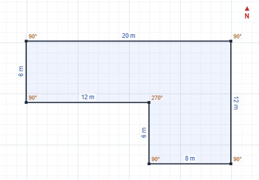
Walls 1–5 were typed as length–bearing pairs. Wall 6 was produced by the Close command, which joins the last corner to the first. Analytically the footprint has area 20 × 12 − 12 × 6 = 168 m², perimeter 64 m, six corners with interior angles of five × 90° and one × 270°, and a building angle of 0° from north.

4.2 Test procedure

All tests were run on the V9.0.14 3D Shadow Analysis module code, loaded in a test page and driven by an automated browser that typed the inputs and clicked exactly as a user would. Results were read back from the simulator's own project export rather than from the drawing tool, so they reflect what the shading engine receives. Four cases were run:

• Case A: the reference house, in metres.
• Case B: a 60′-6″ × 40′ rectangular house entered in feet, with lengths typed in feet-and-inch notation (60'6", 40).
• Case C: a circular arc with a 10 m chord and 3 m sagitta, checked against the geometric formula.
• Case D: a curved wall with a 10 m chord and a typed radius of 7 m, checked for the reported curve length.

4.3 Results

Every transferred quantity matched its analytical value to the reported precision. In Case A the drawing was re-opened from the saved project and showed the same closed outline, 168 m² and 64 m perimeter, confirming that the geometry survives saving and reloading. Case B confirms that the unit layer converts without loss: the house drawn in feet arrives in the shading engine at its exact metric size.

5. Error analysis

The footprint that reaches the shading engine can differ from the surveyed house only through the input route and two deliberate approximations. The bounds below follow directly from the rules in Section 3.

The arc bound follows from the segment rule: when the 4° limit governs (r below about 3.58 m) the deviation is r(1 − cos 2°) ≤ 2.2 mm, and when the 0.25 m chord limit governs it is about 0.25² / (8r), which is again at most 2.2 mm and falls as the radius grows.

Two practical conclusions follow. First, a house entered with typed survey dimensions is transferred to the shading engine without any geometric loss, so the accuracy of the footprint equals the accuracy of the survey. Second, mouse-placed drawing is suitable for sketches and early studies, but a bearing placed by eye can be off by up to 0.25°, so walls that determine the module azimuth should be typed.

6. Discussion and limitations

Survey-native input. Entering each wall as a length and a bearing mirrors how a site engineer records a building with a tape and a compass, and how a closed traverse is computed in surveying. Because the corner angle to the previous wall is displayed while drawing, misread bearings show up immediately as corners that are not 90° where the building is square. The closure check (open ends and the interior-angle sum) then catches dimension errors before any shading is computed.

Independence from imagery. Image tracing ties the footprint to the image's resolution, its north alignment and what is visible from above, where eaves, canopy and shadows can hide the wall line. The drawn footprint avoids all three: north is fixed by construction, the scale is exact, and hidden walls are entered from their measured lengths. The two routes are complementary. Imagery remains the better source for the surroundings, while a drawn plan is the better source for a building whose dimensions are surveyed or taken from an architectural drawing.

Orientation estimate. The quadrupled-angle mean weights each wall by its length, so short returns and bay windows hardly move the result, and a perfectly rectilinear house returns its exact orientation. For buildings that are not rectilinear (for example with 45° or curved walls), the estimate is still a length-weighted compromise. The sun-facing façade and the module azimuth should then be checked, and if necessary set manually.

Limitations.

• One outline per building. The largest closed shape becomes the roof outline. Inner courtyards, separate wings and roof faces at different heights are added afterwards with the module's area and roof-face tools, not from the same drawing.
• Prismatic building. The house is extruded to one height. Pitched roofs, parapets, stair and lift rooms and other rooftop objects must be added with the existing tools for their shading to be modelled.
• Plane geometry. The frame is a flat local plane with north at the top. This is appropriate for a single building; magnetic declination is not applied, so survey bearings must be true (geographic) bearings.
• Arc representation. Curves are stored as polylines. The 360-segment cap applies only to very long arcs and still keeps the deviation below 1 cm for radii up to about 1 km.
• Validation scope. The validation in Section 4 checks geometric transfer against closed-form values. It does not compare simulated shading or energy yield with field measurements, which is a separate validation question for the shading engine itself.
• Snapping trade-off. The magnet towards cardinal directions and square corners speeds up typical drawing. For a deliberately skewed wall, the bearing should be typed so that it is not pulled onto the nearest square direction.

7. Conclusion

The layout-drawing method in IST PVSolar Simulator V9.0.14 turns a surveyed house into the footprint of a 3D shadow analysis without geometric loss. Walls are entered as length–bearing pairs with north fixed upward, and outlines are closed and checked by graph traversal and the interior-angle sum. The footprint is transferred as a floating-point roof polygon at an exact map scale, and the building orientation and module azimuth follow from a length-weighted mean of quadrupled wall bearings.

On reference houses with closed-form answers, the footprint area, perimeter, corner angles, orientation and arc geometry reached the shading engine exactly, in metres and in feet. Typed dimensions are therefore limited only by the accuracy of the survey, and the remaining error sources are bounded and small: 0.5 m grid and 0.25° bearing quantisation for mouse-placed walls, and at most 2.2 mm for curved walls. Future work should validate the complete chain, from drawn footprint to simulated shading loss and energy yield, against measured data from instrumented rooftops.

Data and code availability

The drawing method is implemented in the 3D Shadow Analysis module of IST PVSolar Simulator V9.0.14 (Find Loc. → Draw Building Plan). The reference geometries of Section 4 can be reproduced by entering the wall tables given there. Each drawing, its unit and the building height are stored with the simulator's project file.

References

1. Reda, I. and Andreas, A. (2004). Solar position algorithm for solar radiation applications. Solar Energy, 76(5), 577–589. doi:10.1016/j.solener.2003.12.003. Corrigendum: Solar Energy, 81(6), 838 (2007). Record
2. Reda, I. and Andreas, A. (2003, revised 2008). Solar Position Algorithm for Solar Radiation Applications. NREL Technical Report TP-560-34302. NREL SPA page
3. Braden, B. (1986). The surveyor's area formula. The College Mathematics Journal, 17(4), 326–337. doi:10.1080/07468342.1986.11972974
4. Mardia, K. V. and Jupp, P. E. (2000). Directional Statistics. Chichester: John Wiley & Sons. Catalogue record
5. IST SunPower System (2026). IST PVSolar Simulator V9.0.14, 3D Shadow Analysis module: Draw Building Plan and Help documentation. Software version published 28 October 2026.